AmbientConvectionCapacitance (combined)

The Modelica By Example target only shows as a patch figure and a plot towards the bottom of the page (there is no Modelica code shown).

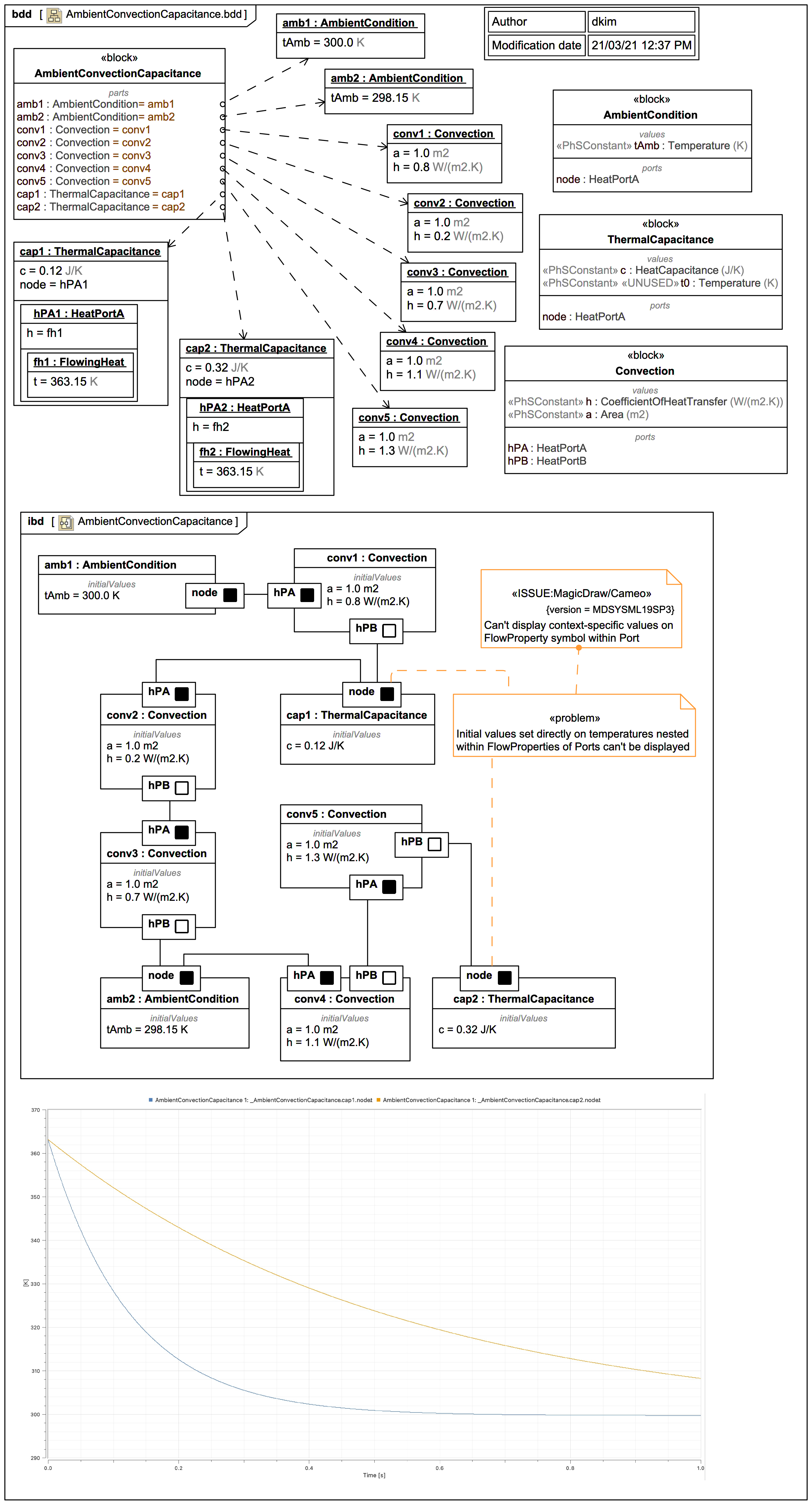
Multiple usages of different components defined in previous slide diagrams are combined in this trail in a block AmbientConvectionCapacitance, which exports via SysPhS to Modelica as:

model AmbientConvectionCapacitance
  AmbientConvectionCapacitance _AmbientConvectionCapacitance;
  model AmbientConvectionCapacitance
    AmbientCondition amb1(tAmb.start=300.0,tAmb.fixed=true);
    AmbientCondition amb2(tAmb.start=298.15,tAmb.fixed=true);
    Convection conv1(a.start=1.0,a.fixed=true,h.start=0.8,h.fixed=true);
    Convection conv2(a.start=1.0,a.fixed=true,h.start=0.2,h.fixed=true);
    Convection conv3(a.start=1.0,a.fixed=true,h.start=0.7,h.fixed=true);
    Convection conv4(a.start=1.0,a.fixed=true,h.start=1.1,h.fixed=true);
    Convection conv5(a.start=1.0,a.fixed=true,h.start=1.3,h.fixed=true);
    ThermalCapacitance cap1(c.start=0.12,c.fixed=true,node.t.start=363.15,node.t.fixed=true);
    ThermalCapacitance cap2(c.start=0.32,c.fixed=true,node.t.start=363.15,node.t.fixed=true);
  equation
    connect(amb1.node,conv1.hPA);
    connect(conv1.hPB,cap1.node);
    connect(cap1.node,conv2.hPA);
    connect(conv2.hPB,conv3.hPA);
    connect(conv3.hPB,amb2.node);
    connect(conv4.hPB,conv5.hPA);
    connect(amb2.node,conv4.hPA);
    connect(conv5.hPB,cap2.node);
  end AmbientConvectionCapacitance;
  model AmbientCondition
    HeatPortA node;
    parameter Temperature tAmb;
  equation
    node.t=tAmb;
  end AmbientCondition;
  model Convection
    parameter CoefficientOfHeatTransfer h;
    parameter Area a;
    HeatPortA hPA;
    HeatPortB hPB;
  equation
    hPA.hFR+hPB.hFR=0;
    hPA.hFR=h*a*(hPA.t-hPB.t);
  end Convection;
  model ThermalCapacitance
    parameter HeatCapacitance c;
    parameter Temperature t0;
    HeatPortA node;
  equation
    c*der(node.t)=node.hFR;
  end ThermalCapacitance;
  connector HeatPortA
    extends HeatFlowElement;
  end HeatPortA;
  connector HeatPortB
    extends HeatFlowElement;
  end HeatPortB;
  connector HeatFlowElement
    flow HeatFlowRate hFR;
    Temperature t;
  end HeatFlowElement;
  type Temperature=Real(unit="K");
  type CoefficientOfHeatTransfer=Real(unit="W/(m2.K)");
  type Area=Real(unit="m2");
  type HeatCapacitance=Real(unit="J/K");
  type HeatFlowRate=Real(unit="J/s");
end AmbientConvectionCapacitance;

There are a few slight difficulties in the SysML/SysPhS modelling. Firstly, recall that: This meant that 'start' values had to be defined directly on the temperature t deep within the Port of each ThermalCapacitance, which is achieved using an instance tree for Context-Specific Values, which is a bit fiddly. The Dependencies from the parts to the instances and instance trees that define the 'start' values are just for illustration.

Unfortunately, a minor tool matter means these Context-Specific Values as applied can't be displayed in the Internal Block Diagram (IBD):

There's a minor inconsistency in the Modelica By Example treatment of Convection. The patch diagrams show only the coefficient of heat transfer h as a variable, the area a is not given, but in the Modelica By Example code the area a is a variable, not a parameter (so not a PhSConstant), and in the Modelica By Example code overrides are always provided, like this:

Convection convection(h=0.7, A=1.0)

In the SysML model here the 'start' for area is assumed to be 1.0 m² for every instance of Convection, which is WET not DRY. One could instead define a shared direct default of 1.0 on the area a within Convection.

Finally, the plot of the temperature on the Ports of each ThermalCapacitance as shown (computed in Wolfram SystemsModeler) looks a tiny bit different from the one shown on the Modelica By Example page.