CoolProp: HOWTO reproduce a pressure vs specific enthalpy chart in Mathematica. Example: R32 refrigerant.

This page identifies a possible issue, concern, error, limitation, or bug!

Webel IT Australia promotes the amazing Mathematica tool and the powerful Wolfram Language and offers professional Mathematica services for computational computing and data analysis. Our Mathematica tips, issue tracking, and wishlist is offered here most constructively to help improve the tool and language and support the Mathematica user community.

DISCLAIMER: Wolfram Research does not officially endorse analysis by Webel IT Australia.

Icon class

icon_class

far fa-sticky-note

icon_class_computed

far fa-sticky-note

Note kind

Policy level

Keywords

Click on the image to view it full size

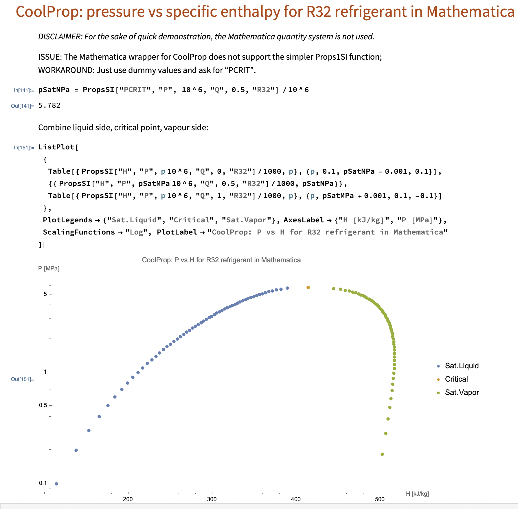
Aim: Reproduce a P-H diagram (pressure vs specific enthalpy, with pressure on the y-axis and specific enthalpy on the x-axes), aka Mollier chart, in Mathematica using CoolProp. Our reference is this R32 refrigerant chart from Daikin.

Dear very practical HVAC&R industry people do please stop calling specific enthalpy just "the enthalpy". Thanks for the frozen food and cool and hot air.

DISCLAIMER: In the following, for the sake of brevity and quick demonstration, the awesome quantity system of Mathematica is not used.

You can't iterate over the specific enthalpy 'H' as explained here:

CoolProp: LIMITATION: DOES NOT accept specific enthalpy 'H' and vapor quality 'Q' as input pairs

Instead, just iterative over P and collect {P,H} points in three regions: the liquid regions "left" of the critical point (with quality Q=0), the critical point itself, and then the vapour region "right" of the critical point.

The Mathematica wrapper for CoolProp does not support the more concise Props1SI function, so instead just use dummy values to obtain 'PCRIT'. In the following, the pressure value is ignored:


pSatMPa = PropsSI["PCRIT", "P", 10^6, "Q", 0.5, "R32"] /10^6

Then just combine the three regions in a ListPlot (with traditional log scaling on the pressure axis):


ListPlot[
 {
  Table[{ PropsSI["H", "P", p 10^6, "Q", 0, "R32"]/1000, p}, {p, 0.1, 
    pSatMPa - 0.001, 0.1}],
  {{ PropsSI["H", "P", pSatMPa 10^6, "Q", 0.5, "R32"]/1000, 
    pSatMPa}},
  Table[{ PropsSI["H", "P", p 10^6, "Q", 1, "R32"]/1000, p}, {p, 
    pSatMPa + 0.001, 0.1, -0.1}]
  },
 PlotLegends -> {"Sat.Liquid", "Critical", "Sat.Vapor"}, 
 AxesLabel -> {"H [kJ/kg]", "P [MPa]"},
 ScalingFunctions -> "Log",
 PlotLabel -> "CoolProp: P vs H for R32 refrigerant in Mathematica"
 ]

The result is shown above in the attached image.

Relates to

Related notes